What is a Phenomenon?
A factor situation that is observed to exist or happen, especially one whose cause or explanation is in question.
- A lightning strike

What is a Phenomenon?
A factor situation that is observed to exist or happen, especially one whose cause or explanation is in question.
- A lightning strike
- A coastline

What is a Phenomenon?
A factor situation that is observed to exist or happen, especially one whose cause or explanation is in question.
- A lightning strike
- A coastline
- A country
What is a Phenomenon?
A factor situation that is observed to exist or happen, especially one whose cause or explanation is in question.
- A lightning strike
- A coastline
- A country
- A dog on a kayak!

Anything and everything are phenomena!
Lightning
A strike is a discrete object, what about a lighting bolt?
- Sort of continuous?
Lightning
A strike is a discrete object, what about a lighting bolt?
- Strike frequency is a continuous field
- Everywhere has a value
- Even the absence of strikes, is a frequency of strikes
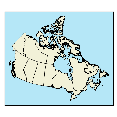
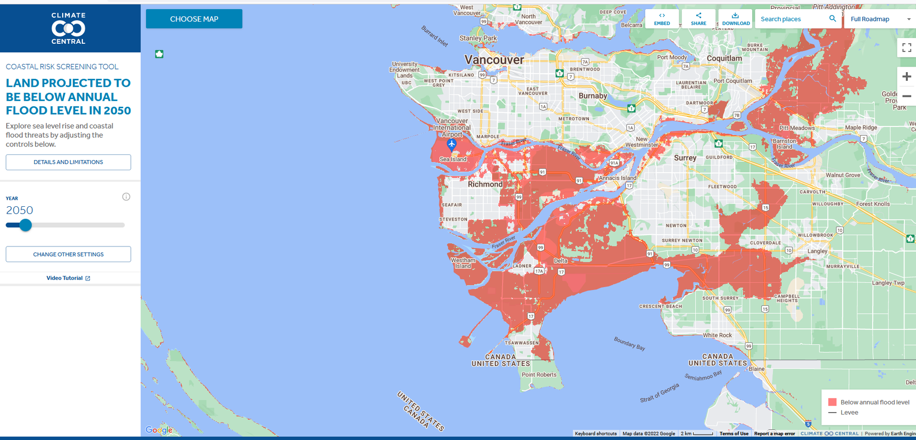
A Coastline
Continuous field at large scale
- Tides & waves
- Where is the exact boundary?
A Coastline
Discrete object at small scale
- Zoom out and the tides/waves don’t really matter
- Its easy to draw a static boundary
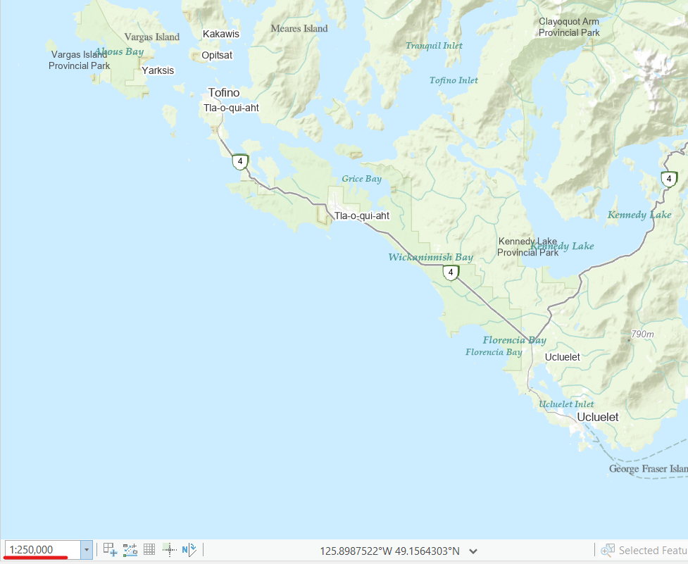
A Coastline
Unless you change the time scale
Discrete Objects
Buildings are a great example.
- Concrete boundaries
- Countable
- Real physical object
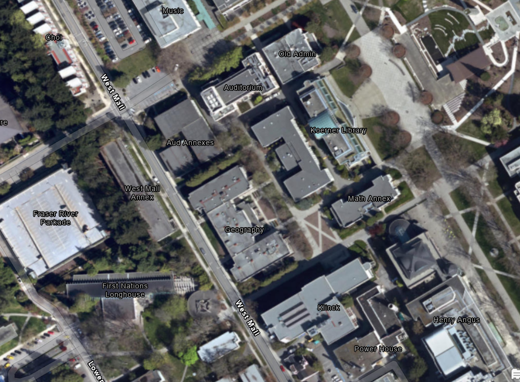
Discrete Objects
Political Boundaries are also a great example.
- Distinct boundaries
- Countable
- Not a physical object
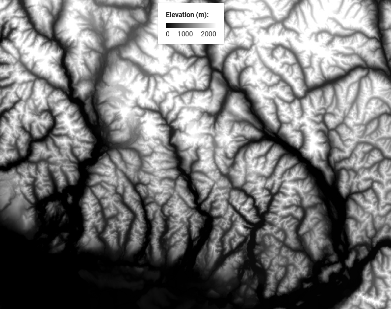
Continuous Fields
Elevation is a great example.
- Everywhere on Earth
- No “number of elevations”
- A physical property
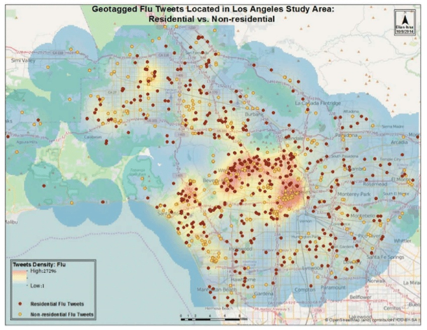
Continuous Fields
Density of tweets is also a great example.
Everywhere has this too
Derived from something countable
But not countable itself
Not a physical property
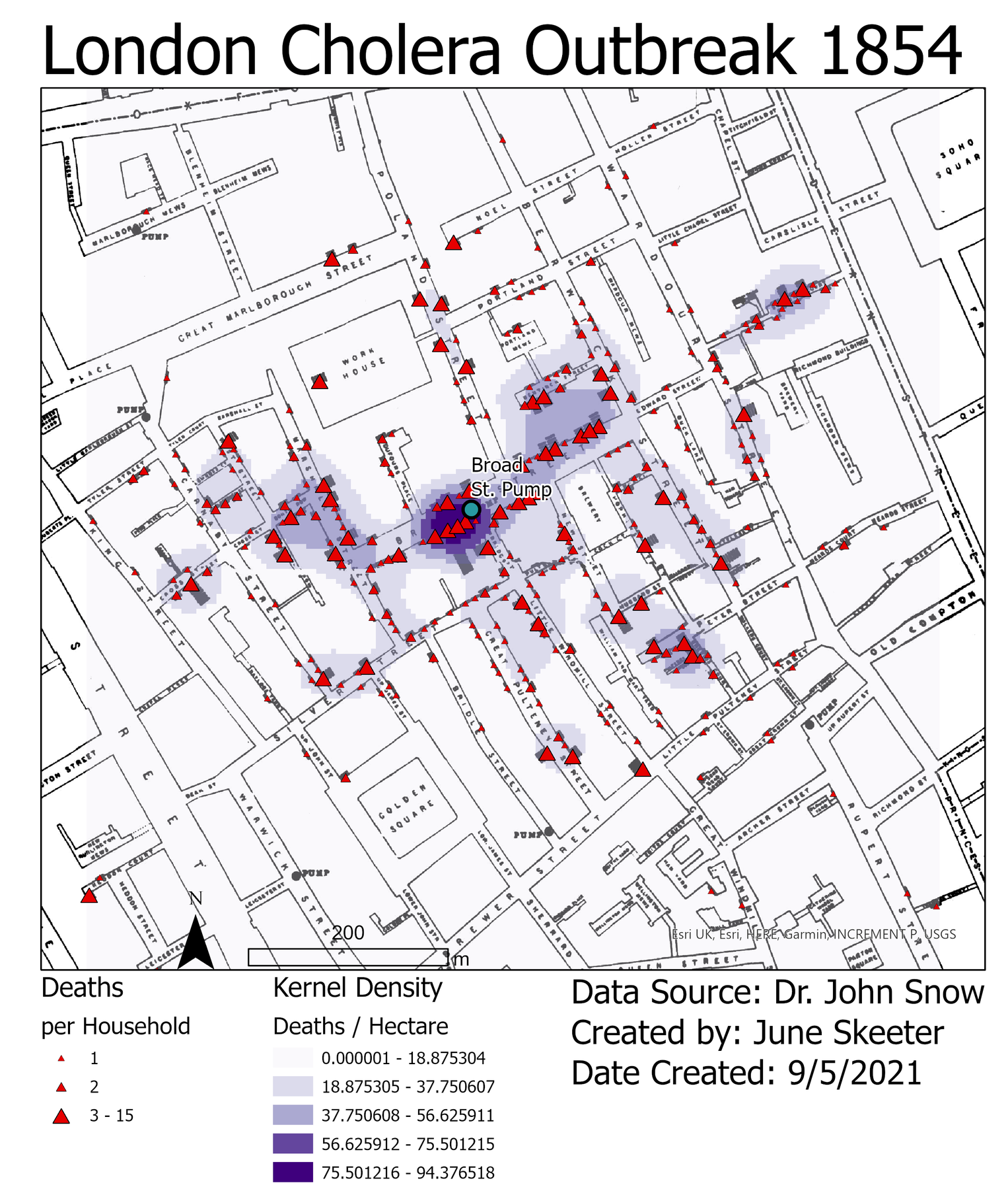
Working Together
Frequently we’ll end up working with both discrete objects and continuous fields.
- In Module 1, you worked with:
- Cholera deaths
- Discrete objects
- Kernel density
- Continuous field
- Cholera deaths
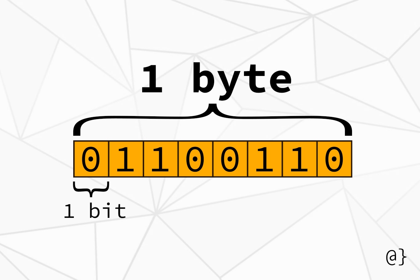
Digital information
Digital information is represented as bits (0’s and 1’s)
- We typically quantify data as bytes (8 bits):
- Kilobyte (kB) = 1,000 bytes
- Megabyte (MB) = 1,000,000 bytes
- Gigabyte (GB) = 1,000,000,000 bytes
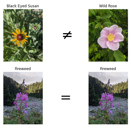
Nominal Scale
Names or categories with no ranking or direction. Categories are not more/less, better/worse, they just different. Some examples include:
- Flower Species
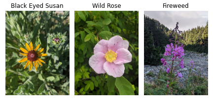
Nominal Scale
Names or categories with no ranking or direction. Categories are not more/less, better/worse, they just different. Some examples include:
- Flower Species
- Zoning Categories
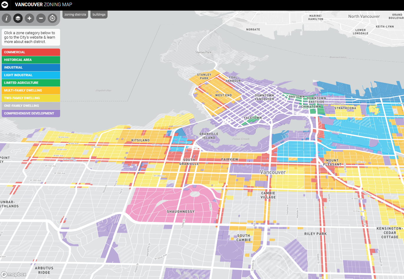
Nominal Scale
Names or categories with no ranking or direction. Categories are not more/less, better/worse, they just different. Some examples include:
- Flower Species
- Zoning Categories
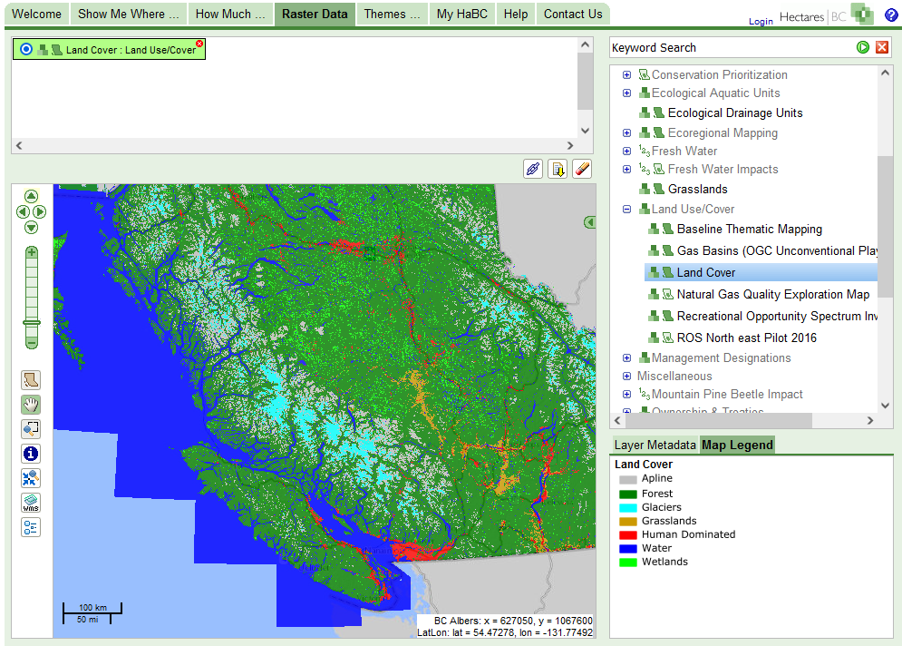
- Land cover Classification
Nominal Operations
With nominal data we can:
- Check equivalency
- Count frequencies
- Nothing else
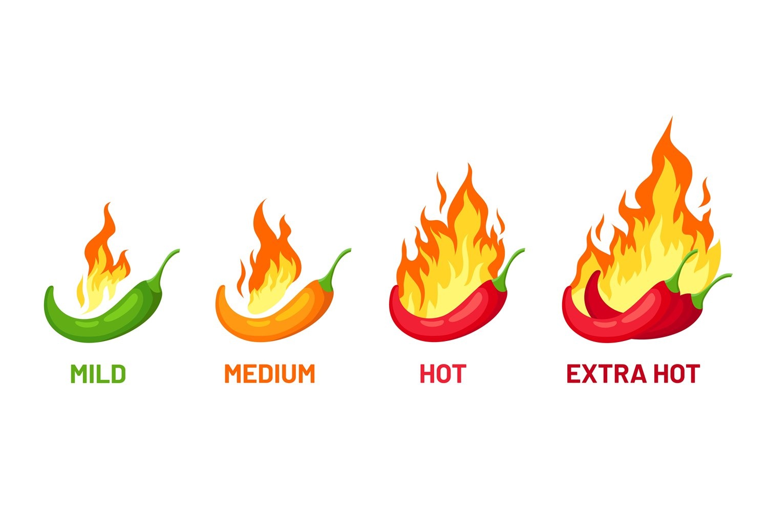
Ordinal Scale
Names or categories with a ranking. The differences are relative. Categories are more/less, better/worse, etc.
- Spice levels
Ordinal Scale
Names or categories with a ranking. The differences are relative. Categories are more/less, better/worse, etc.
- Spice levels
- Relative heights

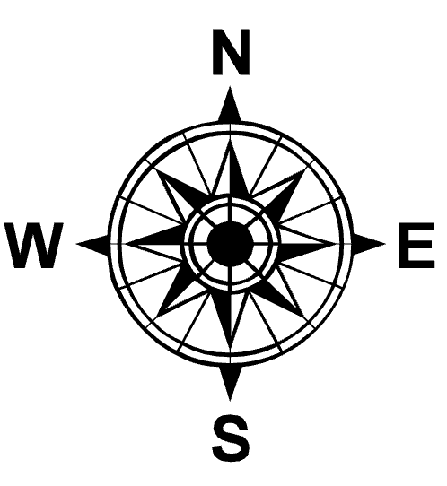
Ordinal Scale
Names or categories with a ranking. The differences are relative. Categories are more/less, better/worse, etc.
- Spice levels
- Relative heights
- Compass Direction
Ordinal Operations
All the same operations as nominal data + more. With ordinal data we can:
- Check equivalency
- Count frequencies
- Check order/rank
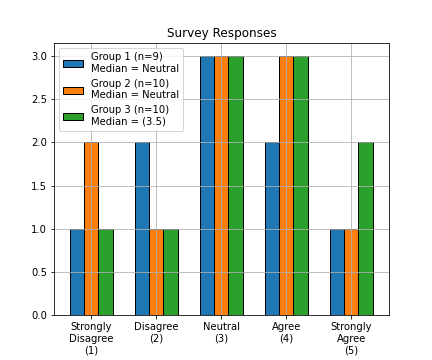
Ordinal Operations
Sometimes we can calculate the median.
- Odd sets the median is the middle.
- Even sets, average of the middle two.
- One solution, arbitrarily assign a numeric score.
Graded Membership
Exceptions that blur the lines. Where to draw the line between forest/alpine?
- Grade membership to assign categories
- Winner take all: alpine meadow
- 45% alpine meadow
- 40% forest
- 5% bare rock

Graded Membership
In practice, lots of qualitative data we work with, especially for natural phenomena, are actually graded membership.
- The downside: variability within the area is lost.
Celsius (interval) vs. Kelvin (ratio)
°C = K-273.15.
- 0 °C: Freezing point of water
- Drops below 0 °C all the time
- 0 K: “Absolute Zero”
- Physically cannot get any colder
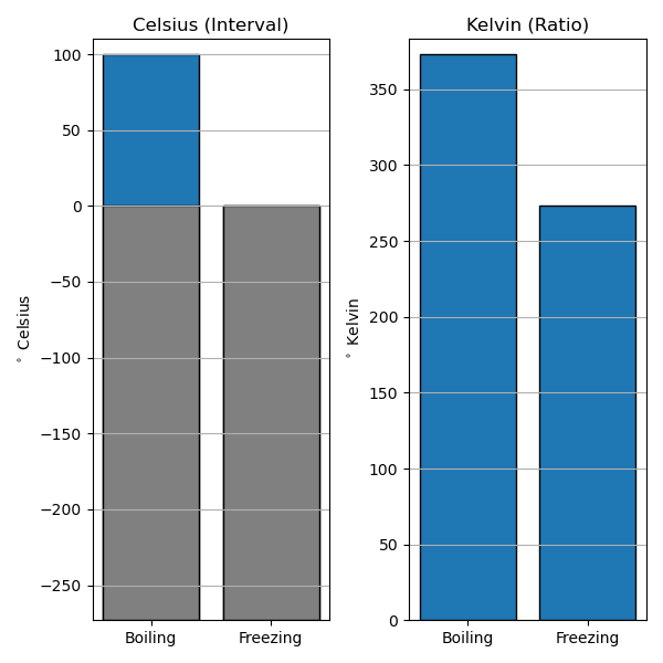
Celsius (interval) vs. Kelvin (ratio)
°C = K-273.15.
- 100 °C is not ∞% warmer than as 0 °C
- It’s actually ~ 36% warmer
- (373.15 K - 273.15 K) ⁄ 273.15 K ~ 0.36
Interval Scale
Interval data has an arbitrary zero point.
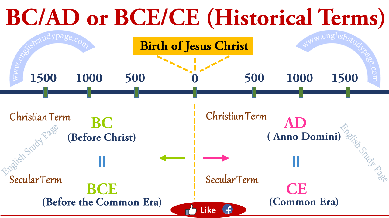
- Calendar years
- Discrete interval data
- Temperature (in celsius)
- Continuous interval data
- Other examples:
- ph scale (continuous)
- Times (discrete-ish)
Interval Scale
Interval data has an arbitrary zero point.
- Calendar years
- Discrete interval data
- Temperature (in celsius)
- Continuous interval data
- Other examples:
- ph scale (continuous)
- Times (discrete-ish)
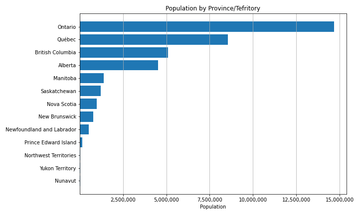
Ratio Scale
Ratio data has a fixed, absolute zero point.
- Population
- Discrete ratio data
- Tree height
- Continuous ratio data
- Other examples:
- Precipitation (Continuous)
- Vote Totals (Discrete)
Ratio Scale
Ratio data has a fixed, absolute zero point.
- Population
- Discrete ratio data
- Tree height
- Continuous ratio data
- Other examples:
- Precipitation (Continuous)
- Vote Totals (Discrete)
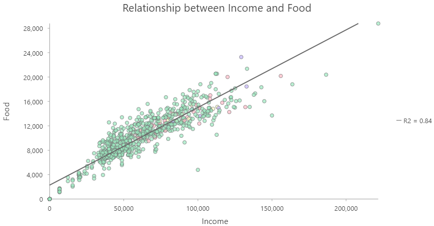
Derived Ratio
In Lab, you are going to work with two derived ratios:
- Income and Food expenditures are correlated
- Need to account for income if you analyze other factors
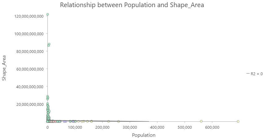
Derived Ratio
In Lab, you are going to work with two derived ratios:
- Population and Area are not highly correlated
- But area definitely influences population
- Need to account for area to analyze other factors
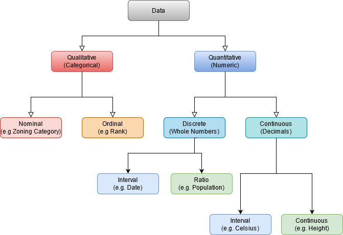
Summary: Types of Data